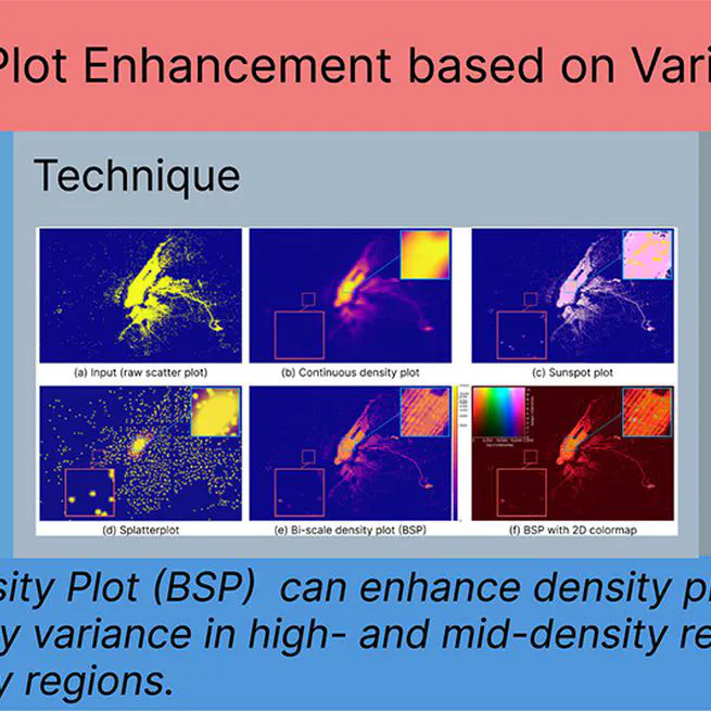
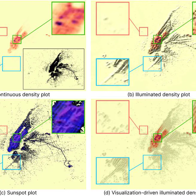
Results Different methods for visualizing the ‘New York TLC Trip’ data with two million points. (a) The scatterplot suffers from overdrawing; overlapping visual marks obscure the major structures. (b) A density plot using a Gaussian kernel reveals the global patterns, but the high density in the center (\ie Manhattan) hides peripheral local structures in the blue box, while outliers in the red box are missed. (c) The Sunspot plot better preserves the outliers but cannot reveal local density variations; see,~\eg the blue box. (d) Splatterplots abstract the density variations in high-density regions, hiding local structures, but show point samples in low-density regions; see the red box. (e) Our Bi-Scale density Plot (BSP) provides more details in low-density regions and reveals more underlying structures; and (f) The BSP enriched by our default 2D colormap, additionally allows looking up and comparing absolute density values and local density variations.
02-09-2025
Results Parameter analysis on the Hertzsprung-Russell diagram dataset [31]. (a,b,c,d) Increasing η makes low-density structures more salient while the high-density structures remain unchanged. (e,f,c,g,h) Decreasing φ makes low-density structures clearer, but at the same time darkens high-density structures.
02-01-2025
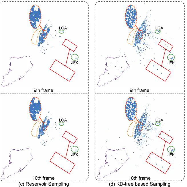
Results Parameter analysis on the Person Activity dataset [16] with the associated PDDr and ESRr scores (see Section 5). The orange dashed boxes and red dashed circles represent typical low- and medium-density regions, respectively. (a,b,c) A large λ results in more regions classified as low-density regions; (d,b,e) a large ω results in more display samples in low-density regions; (f) when λ and ω are both large, almost all low-density regions in the original scatterplot are kept but the data density ratios cannot be maintained; (b,g,h) decreasing stopLevel introduces more display samples; outliers in low-density regions can be shown more clearly but overplotting will have resulted.
01-01-2022
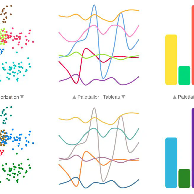
Results Comparison of nearest neighbors definitions in KNN graphs and α-Shape graphs. (a) Results generated by a KNN graph using only point distinctness: the generated colors are hard to discriminate; (b) Nearest neighbors of the selected point in the KNN graph; (c) Results generated by α-Shape graph only using point distinctness: the generated colors are easily to discriminate; (d) Nearest neighbors of the selected point in the α-Shape graph.
01-01-2021
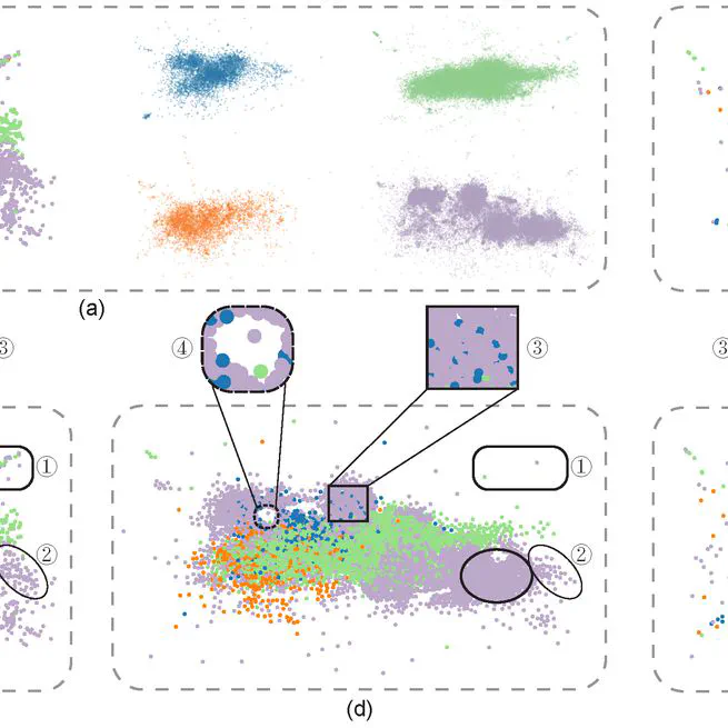
Results Parameter analysis for our method on the Person Activity data set. (a,b,c) Grid size influences the number of point samples. From left to right, the results have 5969, 2273, and 1217 points, respectively. (d,e,f) For a large λ, many outliers become visible, but overdraw happens in dense areas, while a small λ reduces overdraw but miss a few outliers. (g,e,h) A large τ shows too many outliers and regions of medium density are suppressed, while a small τ is more balanced but outliers are reduced. (i) When λ and τ both are large, the overdraw issue becomes severe while showing many outliers.
01-01-2020
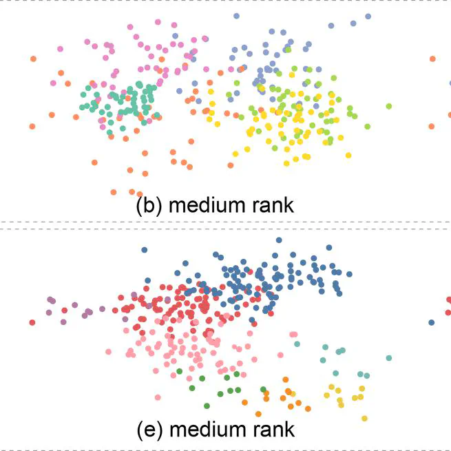
Results Exploring the influence of λ on the selected color assignment: (a) result generated by only considering the color contrast with background; (b) result generated with λ set to 0.1; (c) result generated with λ set to 0.3; and (d) result generated by considering only the point distinctness.
01-01-2019